Matrix Multiplication (Small)

Author: Jie Wang (jiewang@cs.ucla.edu)

This is an example of small-size matrix multiplication. The design files can be found at ${AUTOSA_ROOT}/autosa_tests/mm. The testing environment is summarized in the table below.

Target FPGA	Xilinx Alveo U250
FPGA Synthesis Tools	Xilinx Vivado HLS 2019.2, Xilinx Vitis 2019.2
CPU	Intel(R) Xeon(R) CPU E5-2699 v3 @ 2.30GHz

C Simulation

Run the following example command to generate one design with HLS host code.

./autosa ./autosa_tests/mm/kernel.c \
--config=./autosa_config/autosa_config.json \
--target=autosa_hls_c \
--output-dir=./autosa.tmp/output \
--sa-sizes="{kernel[]->space_time[3];kernel[]->array_part[16,16,16];kernel[]->latency[8,8];kernel[]->simd[2]}" \
--simd-info=./autosa_tests/mm/simd_info.json \
--host-serialize \
--hls

After compilation, you will find all generated files under the directory ${AUTOSA_ROOT}/autosa.tmp/output/src. Copy the hls_script.tcl to the directory autosa.tmp/output.

cp ${AUTOSA_ROOT}/autosa_tests/mm/hls_script.tcl ${AUTOSA_ROOT}/autosa.tmp/output/

Run the TCL script to perform C simulation.

cd ${AUTOSA_ROOT}/autosa.tmp/output/
vivado_hls -f hls_script.tcl

You should see Passed printed out in your terminal showing that C simulation is performed successfully.

RTL Simulation

If you need to verify the design using RTL simulation. There are two more jobs to do.

Modify the Kernel Code

Open the kernel code ${AUTOSA_ROOT}/autosa.tmp/output/src/kernel_kernel.cpp. Locate to the top function void kernel0(A_t16 *A, B_t16 *B, C_t16 *C). You should see the following directives for mapping three global pointers to different AXI buses.

#pragma HLS INTERFACE m_axi port=A offset=slave bundle=gmem_A
#pragma HLS INTERFACE m_axi port=B offset=slave bundle=gmem_B
#pragma HLS INTERFACE m_axi port=C offset=slave bundle=gmem_C

To run RTL simulation, we will need to assign the depth of each AXI bus explictly. Refer to the host code kernel_host.cpp for the size of each array. As we have applied host serialization, the array size might be slightly larger than the original array. In this example, the array A, B, C are allocated with sizes of 16384, 16384, and 4096. Since each array is packed by 16 elements, the depths of each array are 16384/16=1024, 16384/16=1024, 4096/16=256, respectively. Modify the directives above to:

#pragma HLS INTERFACE m_axi port=A offset=slave bundle=gmem_A depth=1024
#pragma HLS INTERFACE m_axi port=B offset=slave bundle=gmem_B depth=1024
#pragma HLS INTERFACE m_axi port=C offset=slave bundle=gmem_C depth=256

Modify the TCL script

Open the TCL script hls_script.tcl. Uncomment the last a few steps:

csim_design
csynth_design
cosim_design

• csim_design is for C simulation.

• csynth_design is for C synthesis that synthesizes C code to RTL.

• cosim_design is for RTL simulation.

We have also provided two more options in the TCl script.

• cosim_design -trace_level all is for RTL simulation while dumping out all waveforms.

• cosim_design -setup -trace_level all is for RTL simulation that only prepares the simulation scripts without actually launching the simulation.

Now run the TCL script again.

vivado_hls -f hls_script.tcl

We will perform C simulation, C synthesis, RTL simulation in order. It will take a few minutes to finish the entire flow. You should be able to see the following information printed in your terminal showing that RTL simulation finishes successfully.

INFO: [COSIM 212-1000] *** C/RTL co-simulation finished: PASS ***

Bitstream Generation

If you need to generate the bitstream for on-board testing, simply remove the --hls flag from the previous AutoSA command.

./autosa ./autosa_tests/mm/kernel.c \
--config=./autosa_config/autosa_config.json \
--target=autosa_hls_c \
--output-dir=./autosa.tmp/output \
--sa-sizes="{kernel[]->space_time[3];kernel[]->array_part[16,16,16];kernel[]->latency[8,8];kernel[]->simd[2]}" \
--simd-info=./autosa_tests/mm/simd_info.json \
--host-serialize

Now instead of HLS host code, an OpenCL host code is generated.

We have prepared a template Makefile for Xilinx Vitis tools.

cp ${AUTOSA_ROOT}/autosa_tests/mm/Makefile ${AUTOSA_ROOT}/autosa.tmp/output/
cp ${AUTOSA_ROOT}/autosa_tests/mm/connectivity.cfg ${AUTOSA_ROOT}/autosa.tmp/output/

Set the proper PLATFORM in the Makefile. By default, we set it to xilinx_u250_xdma_201830_2. You may notice that we also copy a file connectivity.cfg here. This file assigns the DDR bank mapping for the design. By default, we map pointers A, B, C to DDR bank 0, 1, 2. Lastly, modify the MODE in the Makefile for performing different tasks.

• sw_emu: C simulation

• hw_emu: RTL simulation

• hw: Bitstream generation

Note

When using Vitis flow to perform RTL simulation, nothing needs to change in the source code. You may directly set the MODE to hw_emu and perform RTL simulation. However, by default, we will run the kernel 10 times to collect the average runtime. This may significantly prolong the simulation time. Consider reducing the kernel launching times to 1 before using RTL simulation.

To generate the bitstream, set the MODE to hw and use the command below.

make all

It will take a few hours to finish. After the bitstream is generated, use the following command to run it on-board.

make check

Auto-Tuning

We have provided an auto-tuner in the alpha version. The auto-tuner builds analytical models for resource usage and latency. Based on these models, the auto-tuner looks for designs with the least latency under the resource constraints.

Training Resource Models

To use the auto-tuner, the first step is to train te resource models. Run the command below to train the resoruce model.

export AUTOSA_ROOT=$(pwd)
python3 ./autosa_scripts/optimizer.py \
-c './autosa ./autosa_tests/mm/kernel.c --target=autosa_hls_c --simd-info=./autosa_tests/mm/simd_info.json --host-serialize --hls --sa-sizes="{kernel[]->space_time[3]}"' \
--info autosa_config/hw_info.json \
-s autosa_config/optimizer_settings.json \
--train \
-p xilinx

Note

Please don’t forget to set up the environment variable AUTOSA_ROOT to your AutoSA root directory before running the auto-tuner.

The auto-tuner requires a minimal AutoSA compilation command to start. We use the command below.

./autosa ./autosa_tests/mm/kernel.c --target=autosa_hls_c --simd-info=./autosa_tests/mm/simd_info.json --host-serialize --hls --sa-sizes="{kernel[]->space_time[3]}"

As you may notice, we will need to assign the space_time to select the exact dataflow for auto-tuning. This is due to the reason that compiling different dataflows requires some additional flags as we will discuss in the next section. As for now, we use the output-stationary 2D array with the argument --sa-sizes="{kernel[]->space_time[3].

hw_info.json sepecifies the hardware resource constraints of the target FPGA board. optimizer_settings.json is the auto-tuner configuration file. More details about these options are covered in Auto-Tuning (Exhaustive Search).

As the training phase will allocate many temporary files, you may consider adding the flag --tmp-dir to store the intermediate files in some other directories.

Once you launch the auto-tuner in the trainning phase, the auto-tuner will randomly sample the design space and collect a few training samples. These training samples will be synthesized using HLS. We will then build resource models using linear regression with these training samples.

This script will launch multiple processes to synthesize HLS designs. By default, we use 16 processes. The training process takes around 10 minutes to finish on our workstation.

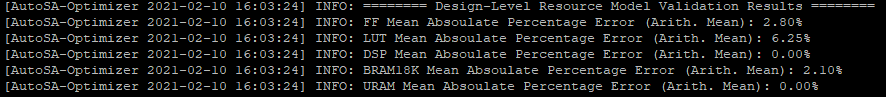
We also evaluate the resource models on the test sets. You will see the resource model accuracy results like below printed on your terminal once this step is finished.

Design Space Exploration

In the next step, we will perform an exaustive search with pruning to find the design with the least latency given the resource constraints. We will improve the DSE with more efficient methods in the future.

The pruning strategies are set in optimizer_settings.json. Details about this file are covered in Auto-Tuning (Exhaustive Search). Depending on the hardware and application, the pruning strategies might be changed. We provide an example file for this application in ${AUTOSA_ROOT}/autosa_config/optimizer_settings_libs/mm_small.json.

Now use the following command to perform DSE.

python3 ./autosa_scripts/optimizer.py \
-c './autosa ./autosa_tests/mm/kernel.c --target=autosa_hls_c --simd-info=./autosa_tests/mm/simd_info.json --host-serialize --hls --sa-sizes="{kernel[]->space_time[3]}"' \
--info autosa_config/hw_info.json \
-s autosa_config/optimizer_settings_libs/mm_small.json \
--search \
-p xilinx

This script will launch multiple processes to search the design space. By default, we use 32 processes. The searching process takes around 3 minutes on our workstation.

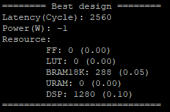
You should see the detailed information about the best design printed out in your terminal like below.

The auto-tuner will dump out the best design found during the DSE in the file DSE.log. By default, we will record the top-10 designs found by DSE.

Dataflow Exploration

AutoSA can help you explore different dataflow choices. As for matrix multiplication, AutoSA finds six different systolic arrays in total. They use loop pair [i], [j], [k], [i,j], [i,k], [j,k] as space loops, respectively. We show each of them in detail below.

Array 1: [i]

This is a 1D systolic array using the loop i as the space loop. The figure below shows the architecture of this array.

This is an output-stationary array. Elements of matrix C are computed locally inside each PE. Data of matrix B are reused across PEs. Data of matrix A are sent directly into each PE.

Here is an example command to compile such a design. Note that we use kernel[]->space_time[0] to select the first design.

./autosa ./autosa_tests/mm/kernel.c \
--config=./autosa_config/autosa_config.json \
--target=autosa_hls_c \
--output-dir=./autosa.tmp/output \
--sa-sizes="{kernel[]->space_time[0];kernel[]->array_part[32,32,32];kernel[]->latency[8,8];kernel[]->simd[2]}" \
--simd-info=./autosa_tests/mm/simd_info.json \
--host-serialize \
--hls

This command leads to a 1x4 1D systolic array.

Array 2: [j]

As you may expect, this is also an output-stationary array with loop j as the space loop. This array is symmetric to the first array. The figure below shows the detailed architecture.

Elements of matrix C are computed locally inside each PE. Data of matrix A are reused across PEs. Data of matrix B are sent directly to each PE.

Here is an example command to compile such a design. Note that we use kernel[]->space_time[1] to select the second design.

./autosa ./autosa_tests/mm/kernel.c \
--config=./autosa_config/autosa_config.json \
--target=autosa_hls_c \
--output-dir=./autosa.tmp/output \
--sa-sizes="{kernel[]->space_time[1];kernel[]->array_part[32,32,32];kernel[]->latency[8,8];kernel[]->simd[2]}" \
--simd-info=./autosa_tests/mm/simd_info.json \
--host-serialize \
--hls

This command leads to a 1x4 1D systolic array.

Array 3: [k]

This array uses loop k as the space loop. The figure below depicts the array architecture.

This is an input-stationary array. Elements of matrix C are accumulated along the PEs. Data of matrix A and B need to be sent to PEs directly.

Use the command below to generate such a design. We use kernel[]->space_time[2] to select the third design. In addition, as AutoSA has no analysis power for reduction loops. We will also need to provide additional information about the reduction property. Note that we add the argument --local-reduce --reduce-op="+" to let AutoSA know that this design perform the reduction along PEs, and the reduction operator is +.

By default, when searching for SIMD loops, AutoSA only considers the time loops. As the loop k is used as the space loop, we add the flag --simd-touch-space to add space loops into consideration in the previous command.

./autosa ./autosa_tests/mm/kernel.c \
--config=./autosa_config/autosa_config.json \
--target=autosa_hls_c \
--output-dir=./autosa.tmp/output \
--sa-sizes="{kernel[]->space_time[2];kernel[]->array_part[4,32,32];kernel[]->latency[8,8];kernel[]->simd[2]}" \
--simd-info=./autosa_tests/mm/simd_info.json \
--host-serialize \
--hls \
--local-reduce \
--reduce-op="+" \
--simd-touch-space \
--array-contraction

This leads to a 1x2 1D array.

One more thing to notice here is that inside each PE, AutoSA only allocates a single register local_C[1][1] for storing the local elements of array C. This is based on the facts that all time loops are parallel loops which means that the PE never works on the same element again. As we add the flag --array-contraction, AutoSA will successfully apply the array contraction to reduce the local buffer size. You may turn off this optimization by removing the argument --array-contraction. When array contraction is turned off, a local buffer local_C[32][32] is allocated inside each PE.

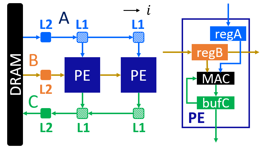
Array 4: [i,j]

This is the 2D output-stationary array as used previously. The figure below shows the detailed architecture.

In this array, data of matrix C are computed locally inside PEs. Data of matrix A are reused horizontally. Data of matrix B are reused vertically.

Below is an example command to compile such a design. Note that we use kernel[]->space_time[3] to select the fourth design.

./autosa ./autosa_tests/mm/kernel.c \
--config=./autosa_config/autosa_config.json \
--target=autosa_hls_c \
--output-dir=./autosa.tmp/output \
--sa-sizes="{kernel[]->space_time[3];kernel[]->array_part[16,16,16];kernel[]->latency[8,8];kernel[]->simd[2]}" \
--simd-info=./autosa_tests/mm/simd_info.json \
--host-serialize \
--hls

This command leads to a 2x2 2D systolic array.

Array 5: [i,k]

This array uses loops i and k as the space loops. The figure below depicts the array architecture.

In this array, data of matrix C are reduced horizontally. Data of matrix B are reused vertically. Data of matrix A are sent directly into each PE.

Use the command below to generate one example array. Note that we use kernel[]->space_time[4] to select the fifth design.

./autosa ./autosa_tests/mm/kernel.c \
--config=./autosa_config/autosa_config.json \
--target=autosa_hls_c \
--output-dir=./autosa.tmp/output \
--sa-sizes="{kernel[]->space_time[4];kernel[]->array_part[32,4,32];kernel[]->latency[16,16];kernel[]->simd[2]}" \
--simd-info=./autosa_tests/mm/simd_info.json \
--host-serialize \
--hls \
--local-reduce \
--reduce-op="+" \
--simd-touch-space \
--array-contraction

This command leads to a 2x2 2D array. Similar as array 3, we add additional information about reduction properties of the application to the compiler. To let AutoSA explore the space loop as SIMD loop, we also add the flag --simd-touch-space. And we add --array-contraction to reduce the local buffer size.

Array 6: [j,k]

This array uses loops i and k as the space loops. The figure below depicts the array architecture. This architecture is symmetric to array 5.

In this array, data of matrix C are reduced horizontally. Data of matrix A are reused vertically. Data of matrix B are sent directly into each PE.

Use the command below to generate one example array. Note that we use kernel[]->space_time[5] to select the fifth design.

./autosa ./autosa_tests/mm/kernel.c \
--config=./autosa_config/autosa_config.json \
--target=autosa_hls_c \
--output-dir=./autosa.tmp/output \
--sa-sizes="{kernel[]->space_time[5];kernel[]->array_part[32,4,32];kernel[]->latency[16,16];kernel[]->simd[2]}" \
--simd-info=./autosa_tests/mm/simd_info.json \
--host-serialize \
--hls \
--local-reduce \
--reduce-op="+" \
--simd-touch-space \
--array-contraction

This command leads to a 2x2 2D array.